Post-processing LakeEnsemblR

Once LakeEnsemblR did successfully run all lake models, you can either extract the output data from the netcdf file for custom analysis and plotting, or use post-processing scripts for an initial look at the output.

Quick post-processing

# define path to the LakeEnsemblR netcdf output
ens_out <- "output/ensemble_output.nc"

# Plot depth and time-specific results
p <- plot_ensemble(ncdf = ens_out, model = c('FLake', 'GLM',  'GOTM', 'Simstrat', 'MyLake'), depth = 0.9,
              var = 'watertemp', date = as.POSIXct("2010-06-13", tz = "UTC"), boxwhisker = TRUE, residuals = TRUE)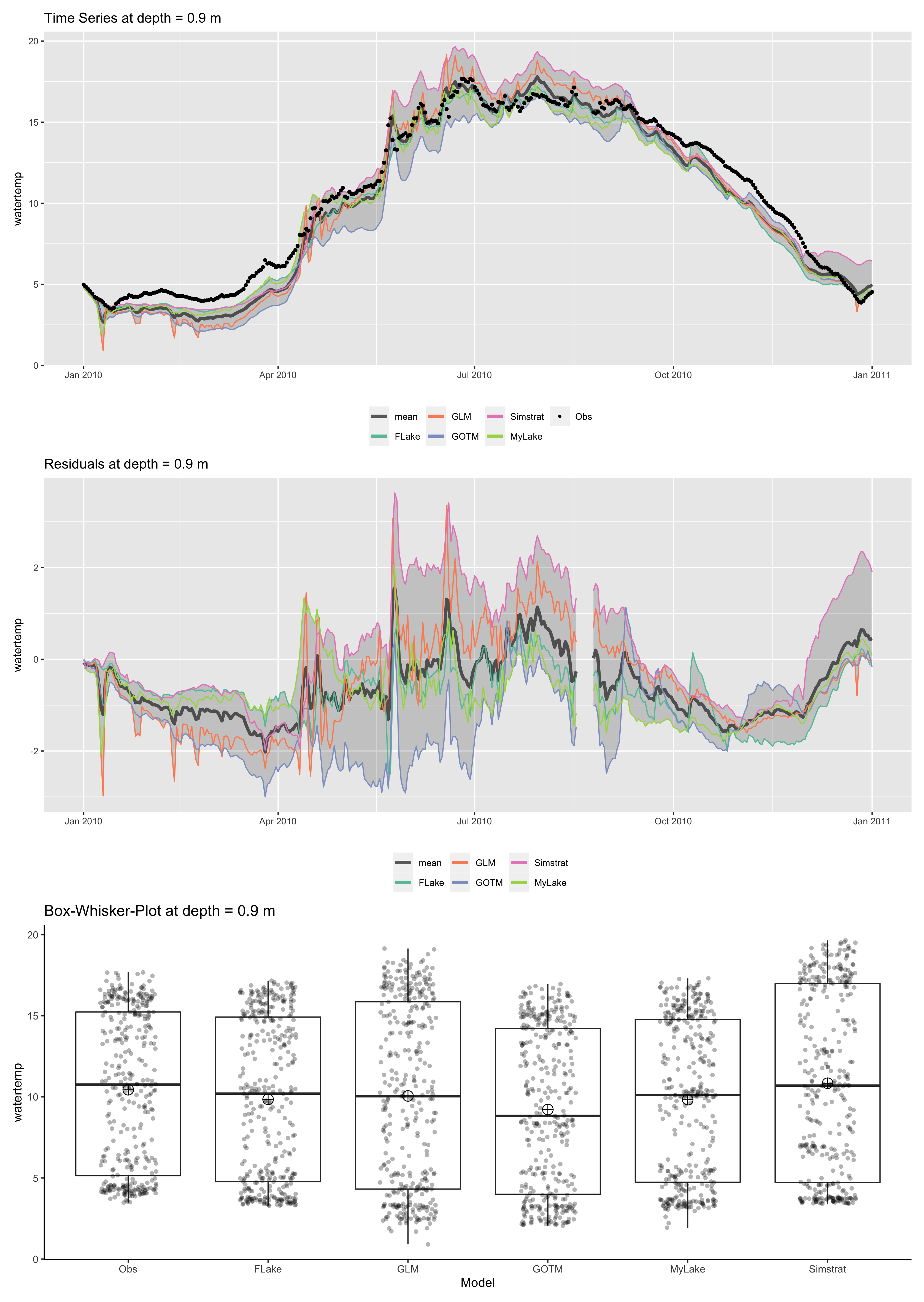

# Take a look at the model fits to the observed data
calc_fit(ncdf = "output/ensemble_output.nc",
         model = c("FLake", "GLM",  "GOTM", "Simstrat", "MyLake"),
         var = "watertemp")

print(calc_fit)
$FLake
      rmse      nse         r         re      nmae
1 3.356338 0.651542 0.6452533 -0.1836044 0.1877008

$GLM
      rmse       nse         r         re      nmae
1 2.677758 0.5880857 0.8791993 -0.2142704 0.2230113

$GOTM
      rmse       nse         r         re      nmae
1 2.855198 0.5303783 0.8983338 -0.2464723 0.2478081

$Simstrat
      rmse        nse        r         re      nmae
1 4.111067 0.02639042 0.653375 -0.2212801 0.2915025

$MyLake
      rmse       nse         r         re      nmae
1 2.548408 0.6258777 0.9059941 -0.1880694 0.1946865

# Take a look at the model performance against residuals, time and depth
plist <- plot_resid(ncdf = ens_out,var = "watertemp",
                   model = c('FLake', 'GLM',  'GOTM', 'Simstrat', 'MyLake'))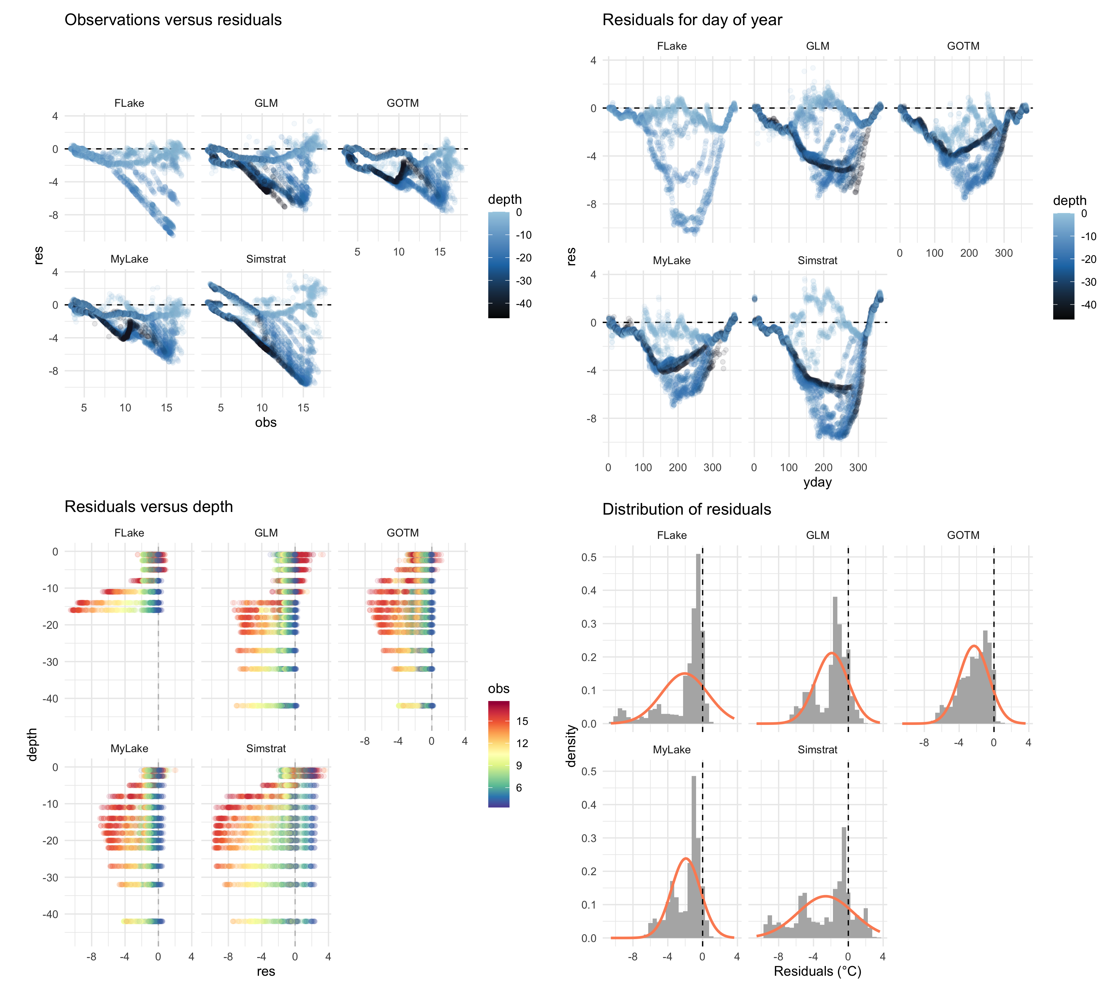

Further custom post-processing

# Load post-processed output data into your workspace
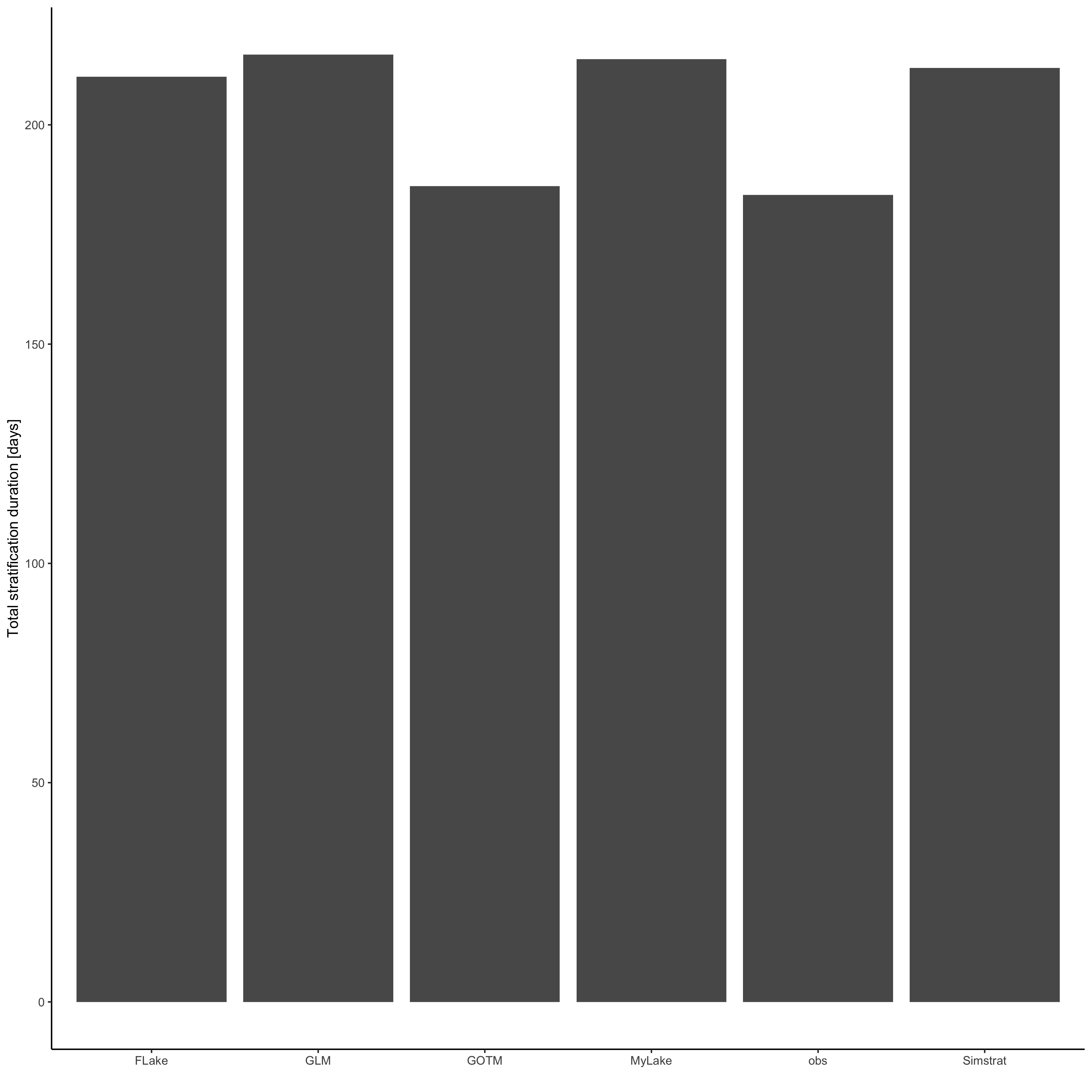
analyse_df <- analyse_ncdf(ncdf = ens_out, spin_up = NULL, drho = 0.1)

# Example plot the summer stratification period
strat_df <- analyse_df$strat

p <- ggplot(strat_df, aes(model, TotStratDur)) +
  geom_col() +
  ylab("Total stratification duration [days]") +
  xlab("") +
  theme_classic()
ggsave("output/model_ensemble_stratification.png", p,  dpi = 300, width = 284, height = 284, units = "mm")