LakeEnsemblR: Basic Use and Sample Applications

Included models

LakeEnsemblR currently includes the following models: GLM (Hipsey et al. (2019)), FLake (Mironov (2008)), GOTM (Umlauf, Bolding, and Burchard (2005)), Simstrat (Goudsmit et al. (2002)), and MyLake (Saloranta and Andersen (2007)).

Introduction

LakeEnsemblR is an R package that lets you run multiple one-dimensional physical lake models.

The settings for a model run are controlled by one centralised, “master” configuration file in YAML format. In this configuration file, you can set all the specifications for your model run, including start and end time, time steps, links to meteorological forcing and bathymetry files, etc. The package then converts these settings to the configuration files required by each model, through the export_config function. This sets up all models to run with the settings specified by the user, and the models are then run through the run_ensemble function. A netcdf file is created with the outputs of all the models, and the package provides functions to extract and plot this data.

Part of the design philosophy of LakeEnsemblR is that all input is given in a standardized format. This entails standard column names (which includes units), comma-separated ASCII files, and a DateTime format using the format YYYY-mm-dd HH:MM:SS, for example 2020-04-03 09:00:00. In this document, we will explain what the required files are and in what format they need to be. We also advise you to look at the provided example files, and at the templates provided with the R package (to be found in package/inst/extdata, or extracted by the function get_template).

Installation

The code of LakeEnsemblR is hosted on the AEMON-J Github page (https://github.com/aemon-j/LakeEnsemblR), and can be installed using the devtools package

devtools::install_github("aemon-j/LakeEnsemblR)

The package relies on multiple other packages that also need to be installed. Most notably, to run the multiple models, it requires the packages FLakeR, GLM3r, GOTMr, SimstratR, and MyLakeR. These packages run the individual models, and contain ways of running the models for the platforms Windows, MacOS, or Linux, through either executables, or by having the model code in R.

The LakeEnsemblR configuration file

In this section, we go through the LakeEnsemblR configuration file. This file controls the settings with which the models are run. It is written in YAML (Yaml Ain’t Markup Language) format, and can be opened by text-editors such as Notepad or Notepad++. Although not needed to use LakeEnsemblR, you can read this file into R with the configr package (read.config function). Within LakeEnsemblR, we provide the get_yaml_multiple and input_yaml_multiple functions to get and input values into this file type.

There is an LakeEnsemblR configuration file provided in the example dataset in the package (LakeEnsemblR::get_template("LakeEnsemblR_config")) or you can download a copy from GitHub here.

Location

The first section is “Location”. Here you specify the name, latitude and longitude, elevation, maximum depth, and initial depth.

You also need to provide a link to the hypsograph (i.e. surface area per depth) file. As in the rest of the configuration file, all links to files are relative to the folder argument in the LakeEnsemblR (from now on: LER) functions (default is the R working directory). We strongly advise to set the working directory to the location of the LER config file, and link to the files relative to this directory (we explain this further in the chapter “Workflow” of this vignette). For example, if your hypsograph file is called hypsograph.csv and in the same folder as the LER config file, the corresponding line in the LER config file would look like

  hypsograph: hypsograph.csv

The data needs to be a comma-separated file (.csv) where 0m is the surface and all depths are reported as positive, in meters. Area needs to be in meters squared. The column names must be Depth_meter and Area_meterSquared

Example of data:

Depth_meter,Area_meterSquared
0,3931000
1,3688025
2,3445050
3,3336093.492
4,3225992.455
5,3133491.11
6,3029720
...

Time

In the “Time” section, you fill in the start and end date of the simulation, and the model time step. time_step indicates the model integration time step, i.e. each time step that the model performs a calculation.

LakeEnsemblR will work with any time zone, provided that the time columns in all input files are in the same time zone and there are no shifts from/to daylight saving time in the files. Of all models, only GLM requires to know the time zone. In LakeEnsemblR this is automatically set to UTC. However, this information is only used in GLM’s albedo_mode 2 and 3, or when GLM’s rad_mode is set to 5 (i.e. computing shortwave radiation if this is not provided). In LakeEnsemblR, the default albedo_mode is 1, and shortwave radiation must be provided, so providing the timezone is not required. Yet if you are changing albedo_mode to 2 or 3, make sure you enter your data in UTC. GOTM also assumes the time to be in UTC, but this is only used when computing shortwave radiation if it is not provided, which does not happen when using LakeEnsemblR.

Config files

In this section, you link to the model-specific configuration files. Templates of these can be found in in the package (get_template("FLake_config"), get_template("GLM_config"), etc. all available templates can be shown using get_template()) or you can download a copy from GitHub here. The setup of LakeEnsemblR is such that you will usually not have to access these files, as most settings are regulated through the LER “main” config file. However, should you want to change some of the more specialised settings in each model, that is possible.

Observations

If you have observations of water temperature, ice cover or water level, you can fill them in here. These will be used in plotting, and in case of water temperature potentially in initialising the temperature profile at the start of the simulation (see next section).

For water temperature, the data needs to be a comma separated values (.csv) file where the datetime column is in the format YYYY-mm-dd HH:MM:SS. Depths are positive and relative to the water surface. Water temperature is in degrees Celsius. The column names must be datetime, Depth_meter and Water_Temperature_celsius (templates available).

Example of data:

datetime,Depth_meter,Water_Temperature_celsius
2004-01-05 00:00:00,0.9,6.97
2004-01-06 00:00:00,2.5,6.71
2004-01-07 00:00:00,5,6.73
2004-01-08 00:00:00,8,6.76
...

For ice height, the data must also be a comma separated values (.csv) file, with datetime column in format YYYY-mm-dd HH:MM:SS and has the column name datetime. Ice height must be provided in meters and the column must be named Ice_Height_meter.

Example of data:

datetime, Ice_Height_meter
2004-01-01 00:00:00,0.3
2004-01-02 00:00:00,0.3
2004-01-03 00:00:00,0.35
...

For water level, the data must also be a comma seperated values (.csv) file, with datetime column in format YYYY-mm-dd HH:MM:SS and has the column name datetime. Water level must be provided in meters above ground and the column must be named Water_Level_meter.

Example of data:

datetime, Water_Level_meter
2004-01-01 00:00:00,45.4
2004-01-02 00:00:00,45.6
2004-01-03 00:00:00,45.7
...

Input

In the “Input” section, you give information about the initial temperature profile, meteorological forcing, the light extinction coefficient, and whether the ice modules should be used.

Firstly, you can give the initial temperature profile with which to start the simulation (link to .csv file with headers Depth_meter, Water_Temperature_celsius, template available using get_template("Initial temperature profile")). If you leave it empty, the water temperature observations will be used, provided you have an observation on the starting time of your simulation.

Secondly, you give the link to the file with your meteorological data. The data needs to be a comma separated values (.csv) file where the datetime column is in the format YYYY-mm-dd HH:MM:SS. See Table 1 for the list of variables, units and column names. The time_zone setting has not been implemented yet.

Table 1. Description of meteorological variables used within LakeEnsemblR with units and required column names.
Description	Units	Column.Name	Status
Downwelling longwave radiation	W/m2	Longwave_Radiation_Downwelling_wattPerMeterSquared	If not provided,it is calculated internally from air temperature, cloud cover and relative humidity/dewpoint temperature
Downwelling shortwave radiation	W/m2	Shortwave_Radiation_Downwelling_wattPerMeterSquared	Required
Cloud cover		Cloud_Cover_decimalFraction	If not provided,it is calculated internally from air temperature, short-wave radiation, latitude, longitude, elevation and relative humidity/dewpoint temperature
Air temperature	°C	Air_Temperature_celsius	Required
Relative humidity	%	Relative_Humidity_percent	If not provided,it is calculated internally from air temperature and dewpoint temperature
Dewpoint temperature	°C	Dewpoint_Temperature_celsius	If not provided,it is calculated internally from air temperature and relative humidity
Wind speed at 10m	m/s	Ten_Meter_Elevation_Wind_Speed_meterPerSecond	Either wind speed or u and v vectors is required
Wind direction at 10m	°	Ten_Meter_Elevation_Wind_Direction_degree	Not required, but if provided u and v vectors are calculated internally
Wind u-vector at 10m	m/s	Ten_Meter_Uwind_vector_meterPerSecond	Either wind speed or u and v vectors is required
Wind v-vector at 10m	m/s	Ten_Meter_Vwind_vector_meterPerSecond	Either wind speed or u and v vectors is required
Precipitation	mm/day	Precipitation_millimeterPerDay	Not strictly required but is important for mass budgets in some models.
Precipitation	mm/hr	Precipitation_millimeterPerHour	Different unit option for precipitation.
Rainfall	mm/day	Rainfall_millimeterPerDay	If not provided,it is calculated internally from precipitation
Rainfall	mm/hr	Rainfall_millimeterPerHour	Different unit option for rainfall.
Snowfall	mm/day	Snowfall_millimeterPerDay	If not provided, it is calculated internally from rain or precipitation when air temperature < 0 degC
Snowfall	mm/hr	Snowfall_millimeterPerHour	Different unit option for snowfall.
Sea level pressure	Pa	Sea_Level_Barometric_Pressure_pascal	Not required
Surface level pressure	Pa	Surface_Level_Barometric_Pressure_pascal	Is calculated from sea level pressure if not provided
Vapour pressure	mbar	Vapour_Pressure_milliBar	If not provided,it is calculated internally from air temperature and relative humidity/dewpoint temperature

Next you can either give a value for Kw (light extinction coefficient) in 1/m, or give the link to a file, where you can vary Kw over time (template available using get_template("Light extinction")). The file must be a comma-separated file (.csv) with the two columns datetime and Extinction_Coefficient_perMeter containing the date in the format (YYYY-mm-dd HH:MM:SS) and corresponding Kw value in 1/m.

Lastly, you can specify if you want to use the ice modules that are present in some of the models.

Inflows

Specify if you want to add inflows to your simulation. If yes, you need to link to a file with the inflow data. The data needs to be a comma separated values (.csv) file where the datetime column is in the format YYYY-mm-dd HH:MM:SS. Flow discharge, water temperature, and salinity need to be specified. The column names must be datetime, Flow_metersCubedPerSecond, Water_Temperature_celsius, and Salinity_practicalSalinityUnits (template available using get_template("Inflow") ). If you have multiple inflows, you should add suffixes “_1”, “_2”, etc. The fix_wlvl argument lets you fix the water level in the GOTM model, to reproduce the behaviour of an earlier version of LakeEnsemblR.

Example of inflow data:

datetime,Flow_metersCubedPerSecond,Water_Temperature_celsius,Salinity_practicalSalinityUnits
2005-01-01 00:00:00,5.62,6.96,0.00
2005-01-02 00:00:00,2.32,6.00,0.00
2005-01-03 00:00:00,1.77,8.44,0.00
2005-01-04 00:00:00,4.64,7.27,0.00
...

Outflows

For the models that allow changing water level (at this moment GLM, GOTM, Simstrat) outflows can be set in this section by setting use to true. The outflow discharge must be provided in daily resolution in a .csv file specified by file. The file must contain a date column in YYYY-mm-dd HH:MM:SS format called datetime and for every outflow (specified by number_outflows) one column titled Flow_metersCubedPerSecond, if more than one outflow are defined the outflow columns need to be numbered like this: Flow_metersCubedPerSecond_1, Flow_metersCubedPerSecond_2. For each outflow the depth of the outflow must be specified as height in meters above the lake bottom, or if the outflow is a surface outflow it can be set to “-1”.

outflows:
   use: true                                    # use outflows? [true/false]
   file: LakeEnsemblR_outflow_standard.csv      # file with outflow data
   number_outflows: 2                           # number of outflows in the outflow file
   outflow_lvl:                                 # height of the outflow above the ground.
      - -1
      - 15

Output

In the “Output” section, you specify how the output should look like. This can be “netcdf” or “text”, which will generate a series of csv files in rLakeAnalyzer format. You can specify the depth interval of the output, and the frequency. Also specify what variables should be in the output (currently “temp”, “ice_height”, “salt”, “dens”, and “w_level”).

Scaling factors

In the “Scaling factors” (scaling_factors) section scaling factors to be applied to meteorological input as well as to inflows and outflows, either for all models or model-specific can be defined. If the section is not specified, no scaling is applied. Using “all” scaling factors that should be applied to all models can be defined, otherwise model specific scaling can be supplied by using the model name. If both “all” and model-specific are specified for a certain model, only the model-specific scaling is applied. If there are multiple inflows or outflows a list of scaling parameters for each of them must be provided (see example).

scaling_factors:
   all:
      wind_speed: 1.0
      swr: 1.0
   Simstrat:
      wind_speed: 0.95
   GLM:
     outflow:
      - 1.02
      - 1.03

Model parameters

All models in LakeEnsemblR have different parameterisations. In this section, you can set the value of any parameter in one of the model-specific configuration files.

You can give either only the name of the parameter, but if needed you can also provide the name of the section in which the parameter occurs, separated by a /. For example for GOTM’s k_min parameter:

  GOTM:
    k_min: 3.6E-6

or:

  GOTM:
    turb_param/k_min: 3.6E-6

Calibration

This section is used when calibrating the models. In the package, the cali_ensemble function runs the calibration. For all three methods model specific parameters and scaling factors for the input meteorological forcing can be calibrated. In any case the parameters to be calibrated are definded in the master control .yaml file. The meteo scalings are defined in the met: section and the model specific parameters in sections with the corresponding model names e.g. MyLake:. The meteo scaling names must be the short names for the meteo variables, which are defined in the met_var_dic data and can be inspected using print(met_var_dic). The model specific names must be the parameter name as given in the model specific configuration file (e.g. gotm.yaml) combined with the lowest section name in which the parameter can be found and separated by a slash “/” (e.g. turb_param/k_min). An example of how the calibration section could look like is given below:

calibration:                                   # Calibration section                                   # Calibration section
   met:                                        # Meteo scaling parameter
      wind_speed:                              # Wind speed scaling
         lower: 0.5                            # lower bound for wind speed scaling        
         upper: 2                              # upper bound for wind speed scaling
         initial: 1                            # initial value for wind speed scaling
         log: false                            # log transform scaling factor
      swr:                                     # shortwave radiation scaling
         lower: 0.5                            # lower bound for shortwave radiation scaling
         upper: 1.5                            # upper bound for shortwave radiation scaling
         initial: 1                            # initial value for shortwave radiation scaling
         log: false                            # log transform scaling factor
   Simstrat:                                # Simstrat specific parameters                                 
      a_seiche:
         lower: 0.0008                         # lower bound for parameter
         upper: 0.003                          # upper bound for parameter
         initial: 0.001                        # initial value for parameter
         log: false                            # log transform scaling factor                          
   MyLake:                                  # MyLake specific parameters                                    
     Phys.par/C_shelter:
        lower: 0.14                            # lower bound for parameter
        upper: 0.16                            # upper bound for parameter
        initial: 0.15                          # initial value for parameter
        log: false                             # log transform scaling factor   
   GOTM:                                    # GOTM specific parameters
      turb_param/k_min:
         lower: 5E-4                           # lower bound for parameter
         upper: 5E-6                           # upper bound for parameter
         initial: 1E-5                         # initial value for parameter
         log: true
   GLM:                               # GLM specific parameters
      mixing/coef_mix_hyp:
         lower: 0.1                       # lower bound for parameter
         upper: 2                         # upper bound for parameter
         initial: 1                       # initial value for parameter
         log: false                       # log transform scaling factor
   FLake:                             # FLake specific parameters
      c_relax_C:
         lower: 0.00003                  # lower bound for parameter
         upper: 0.3                      # upper bound for parameter
         initial: 0.003                  # initial value for parameter
         log: true                       # log transform scaling factor

An example on how to run the calibration see section 5.7 “Model calibration”.

Workflow

In this chapter, we quickly show you how your workflow with LakeEnsemblR could look like.

Setting up a directory

First, you make an empty directory for the simulations of a specific lake. In this directory, you place the LakeEnsemblR configuration file, and the necessary LakeEnsemblR-format input files (e.g. meteorology, inflow, water temperature observations, hypsograph). Within this directory, you create empty folders for each model (FLake, GLM, GOTM, Simstrat, MyLake), and in here you place the model-specific configuration files, corresponding the information you put in the config_files section in the LER config file.

Export_config

Then, you run the export_config function, which exports the settings in the LER configuration file to the model-specific configuration files. It is possible to run parts of this function, such as export_meteo, if the meteorological forcing is the only thing you changed, but usually you will run export_config.

Optional: changes in model-specific directories

Optionally, you can now go into the model-specific configuration files and make further changes. This should not be needed for regular simulations, especially since you can control parameters in the model_parameters section of the LER config file, but the option is there. For example, if you want to change the depth of the inflow in the Simstrat model, you could go to the Simstrat folders and make these changes manually (or through a script you wrote). It speaks for itself that these changes should be done only if you are sure this is what you need, and LakeEnsemblR does not provide further support for this.

Run_ensemble

The next step would be to call run_ensemble, which runs all the models. A new folder called “output” is created, in which a netcdf-file will be put with all the results from the model runs. If you are interested, each model sub-folder will also have an “output” folder, with the model-specific model output.

Example model run

See below for an example run, and some post-processing of the data.

# Install packages - Ensure all packages are up to date
devtools::install_github("aemon-j/GLM3r", ref = "v3.1.1")
devtools::install_github("USGS-R/glmtools", ref = "ggplot_overhaul")
devtools::install_github("aemon-j/FLakeR", ref = "inflow")
devtools::install_github("aemon-j/GOTMr")
devtools::install_github("aemon-j/gotmtools")
devtools::install_github("aemon-j/SimstratR")
devtools::install_github("aemon-j/MyLakeR")
devtools::install_github("aemon-j/LakeEnsemblR")

# Load libraries
library(LakeEnsemblR)
library(ggplot2)

# Set working directory with example data from Lough Feeagh, Ireland
template_folder <- system.file("extdata/feeagh", package= "LakeEnsemblR")
dir.create("example") # Create example folder
file.copy(from = template_folder, to = "example", recursive = TRUE)
setwd("example/feeagh") # Change working directory to example folder

# Set models & config file
model <- c("GLM",  "FLake", "GOTM", "Simstrat", "MyLake")
config_file <- "LakeEnsemblR.yaml"

# 1. Example - creates directories with all model setup
export_config(config_file = config_file, model = model, folder = ".")


# 2. Run ensemble lake models
wtemp_list <- run_ensemble(config_file = config_file,
                           model = c("FLake", "GLM", "GOTM", "Simstrat", "MyLake"),
                           return_list = TRUE)

Plotting the model outputs is very easy using the plot_heatmap() function:

g1 <- plot_heatmap("output/ensemble_output.nc")

ggsave("output/model_ensemble_watertemp.png", g1,  dpi = 300,width = 384,height = 300,
       units = "mm")

Post-processing

Once LakeEnsemblR did successfully run all lake models, you can either extract the output data from the netcdf file for custom analysis and plotting, or use post-processing scripts for an initial look at the output.

Quick post-processing

Now that the model simulations are finished, you can extract the data with load_var, or plot it with plot_ensemble. You can extract data from the netcdf file to do any further analysis. The ncdf4 R package supports working with netcdf data in R, and the PyNcView software (https://sourceforge.net/projects/pyncview/) can be used to look at netcdf output.

# Import the LER output into your workspace
ens_out <- "output/ensemble_output.nc"

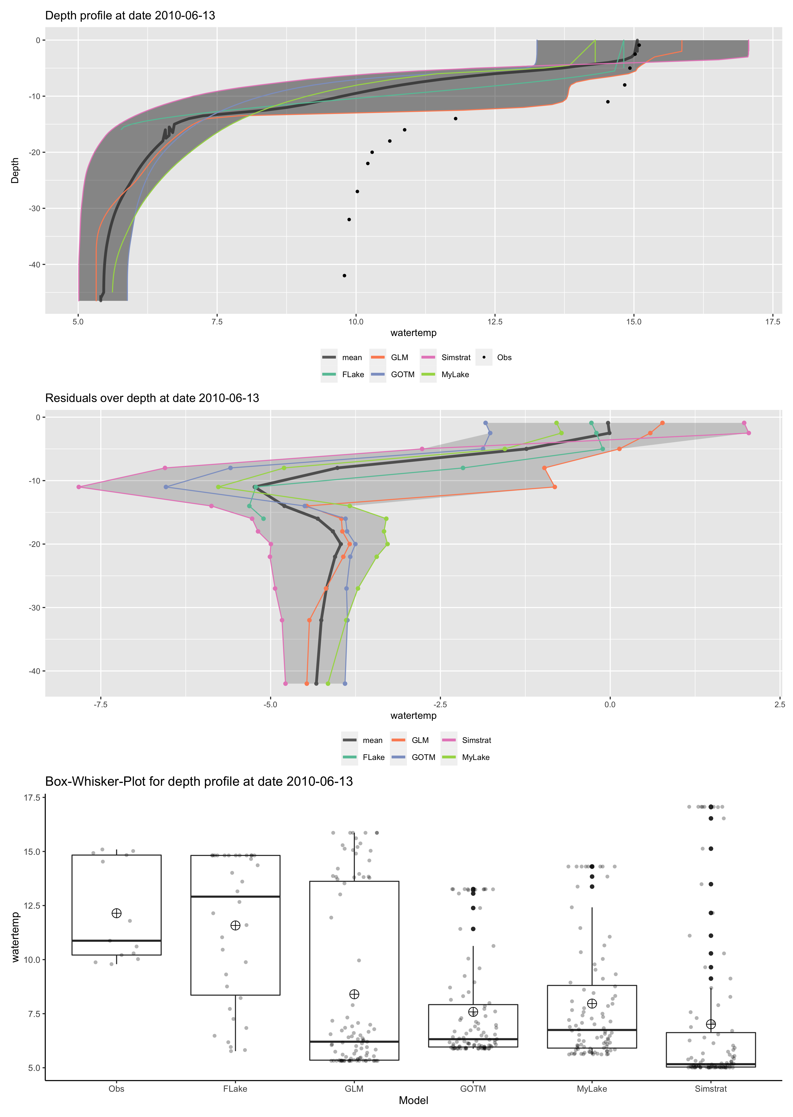
# Plot depth and time-specific results
p <- plot_ensemble(ncdf = ens_out, model = c("FLake", "GLM",  "GOTM", "Simstrat", "MyLake"),
                   depth = 0.9, var = "temp",
                   boxwhisker = TRUE, residuals = TRUE)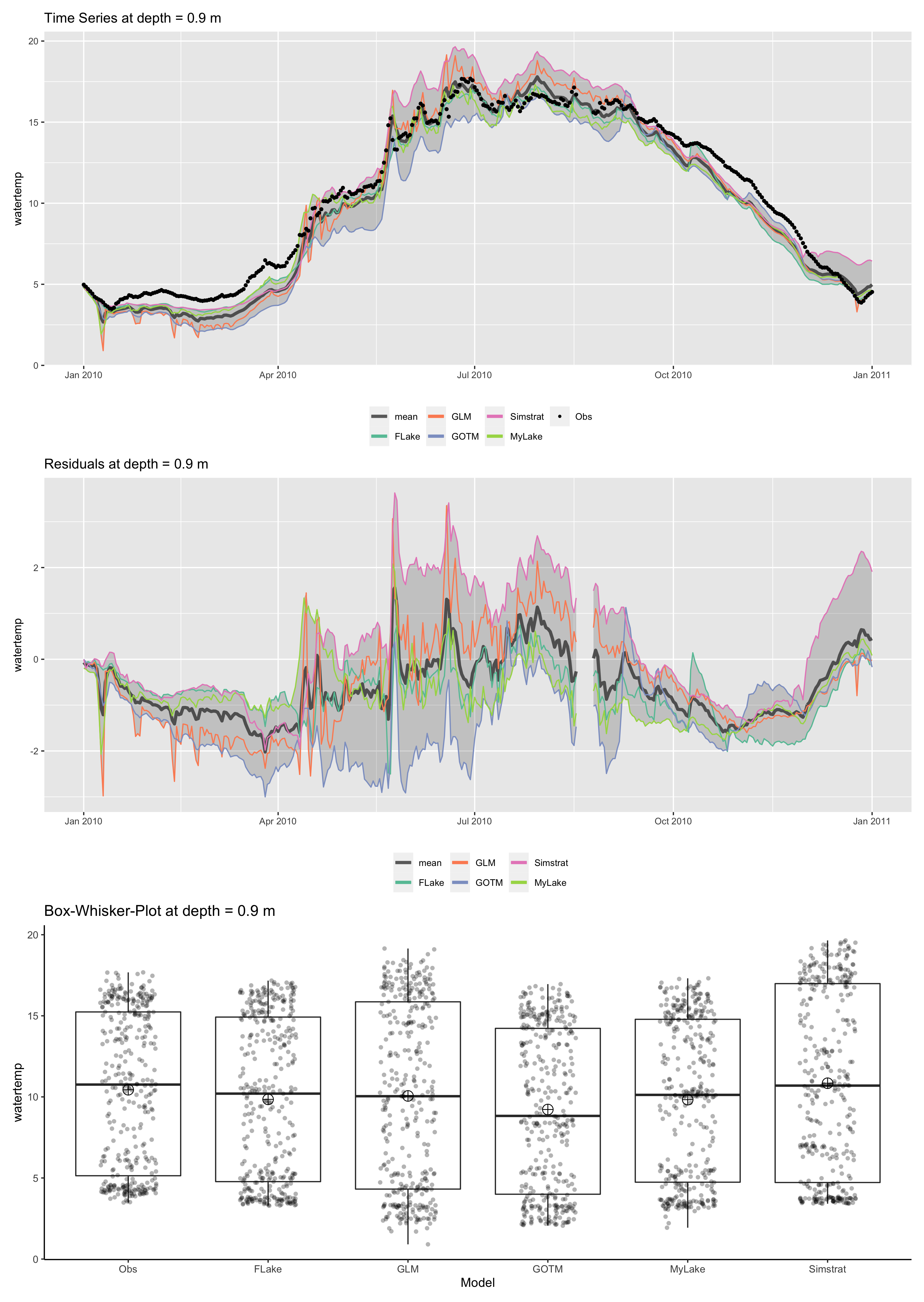

# Take a look at the model fits to the observed data
calc_fit(ncdf = "output/ensemble_output.nc",
         model = c("FLake", "GLM",  "GOTM", "Simstrat", "MyLake"),
         var = "temp")

$FLake
      rmse       nse         r      bias      mae      nmae
1 3.353107 0.6522126 0.6448119 -2.048613 2.090902 0.1863813

$GLM
      rmse       nse         r      bias      mae      nmae
1 2.671799 0.5899169 0.8976564 -2.078693 2.116857 0.2334367

$GOTM
      rmse       nse         r      bias      mae      nmae
1 2.076912 0.7515084 0.9373982 -1.642189 1.691141 0.1990019

$Simstrat
      rmse       nse         r      bias      mae      nmae
1 2.517848 0.6347966 0.8378958 -1.237562 1.983922 0.2224387

$MyLake
      rmse       nse         r      bias      mae      nmae
1 2.548408 0.6258777 0.9059941 -1.922304 1.958271 0.1946865

$ensemble_mean
      rmse       nse         r      bias      mae      nmae
1 2.385461 0.6721914 0.9118315 -1.781649 1.874828 0.1992386

# Take a look at the model performance against residuals, time and depth
plist <- plot_resid(ncdf = ens_out,var = "temp",
                   model = c('FLake', 'GLM',  'GOTM', 'Simstrat', 'MyLake'))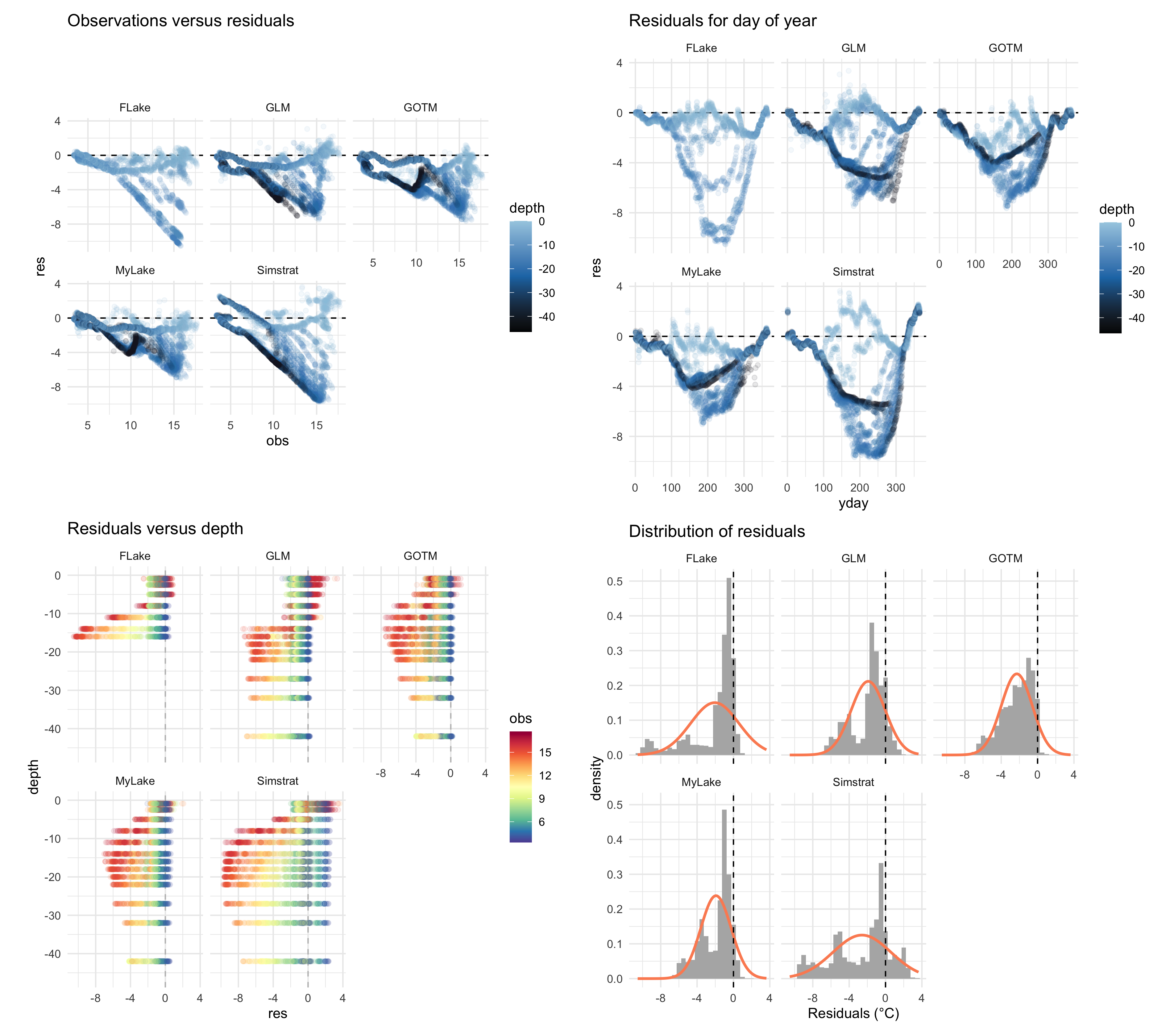

Further custom post-processing

# Load post-processed output data into your workspace
analyse_df <- analyse_ncdf(ncdf = ens_out, model = model, spin_up = NULL, drho = 0.1)

# Example plot the summer stratification period
strat_df <- analyse_df$strat

p <- ggplot(strat_df, aes(model, TotStratDur)) +
  geom_col() +
  ylab("Total stratification duration [days]") +
  xlab("") +
  theme_classic()
ggsave("output/model_ensemble_stratification.png", p,  dpi = 300, width = 284,
       height = 284, units = "mm")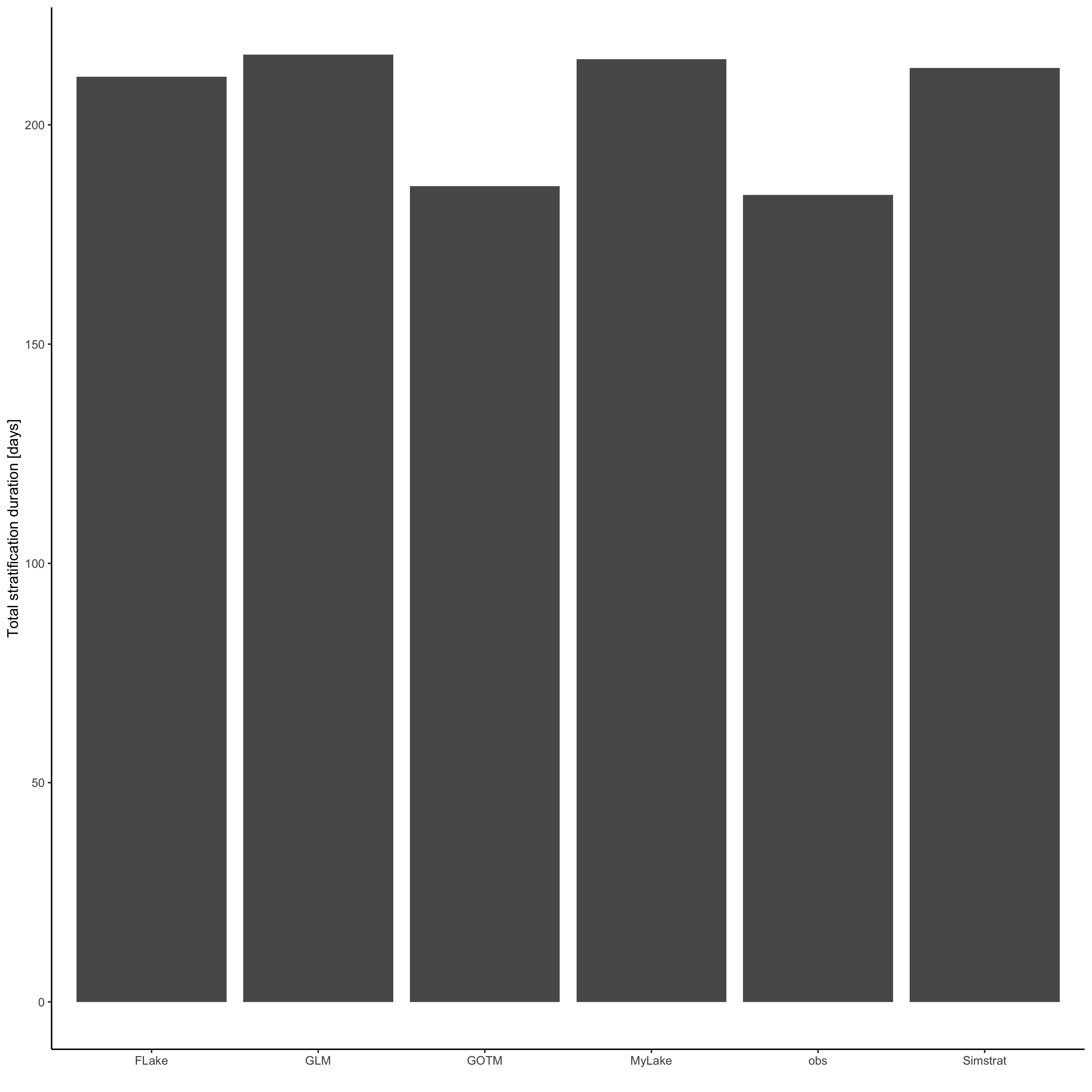

Adding several model runs to a single netcdf file

The run_ensemble function allows to add different model runs to a single netcdf file. This is done by setting the argument add = TRUE. Only model runs that go over the same time period and use the same time steps can be combined to a single netcdf file. Using this functionality e.g. model runs with different parametrizations can be ran and compared. Many diagnostic functions like calc_fit or plot_ensemble have two additional arguments dim and dim_index to select which dimension should be used. The argument dim can either be “model” or “member” and dim_index then gives the index of the other dimension to be used, e.g. if the netcdf file contains 3 different ensemble runs (member) with the two models “FLake” and “GLM” calc_fit("ncfile.nc", model = c("FLake", "GLM"), dim = "model", dim_index = 2) calculates the model performance of both model for the second ensemble run (dim_index = 2). Whereas,
calc_fit("ncfile.nc", model = c("FLake", "GLM"), dim = "member", dim_index = 2) calculates the performance of all model runs (members) of the GLM runs (the second model).

Model calibration

LakeEnsemblR includes some tools for automatic model calibration which are included in the cali_ensemble() function. The function profides three methods:

method “LHC”: Lathin hypercube calibration
method “MCMC”: Markov Chain Monte Carlo simulation using the modMCMC function from the FME package (Soetaert and Petzoldt (2010))
method “modFit”: model fitting using one of the algorithms provided in the modFit function from the FME package (Soetaert and Petzoldt (2010))

For details on the structure of the calibration section in the yaml config file see section 4.11.

calibration:                                   # Calibration section                                   # Calibration section
   met:                                        # Meteo scaling parameter
      wind_speed:                              # Wind speed scaling
         lower: 0.5                            # lower bound for wind speed scaling        
         upper: 2                              # upper bound for wind speed scaling
         initial: 1                            # initial value for wind speed scaling
         log: false                            # log transform scaling factor
      swr:                                     # shortwave radiation scaling
         lower: 0.5                            # lower bound for shortwave radiation scaling
         upper: 1.5                            # upper bound for shortwave radiation scaling
         initial: 1                            # initial value for shortwave radiation scaling
         log: false                            # log transform scaling factor
   Simstrat:                                # Simstrat specific parameters                                 
      a_seiche:
         lower: 0.0008                         # lower bound for parameter
         upper: 0.003                          # upper bound for parameter
         initial: 0.001                        # initial value for parameter
         log: false                            # log transform scaling factor                          
   MyLake:                                  # MyLake specific parameters                                    
     Phys.par/C_shelter:
        lower: 0.14                            # lower bound for parameter
        upper: 0.16                            # upper bound for parameter
        initial: 0.15                          # initial value for parameter
        log: false                             # log transform scaling factor   
   GOTM:                                    # GOTM specific parameters
      turb_param/k_min:
         lower: 5E-6                           # lower bound for parameter
         upper: 5E-4                           # upper bound for parameter
         initial: 1E-5                         # initial value for parameter
         log: true
   GLM:                               # GLM specific parameters
      mixing/coef_mix_hyp:
         lower: 0.1                       # lower bound for parameter
         upper: 2                         # upper bound for parameter
         initial: 1                       # initial value for parameter
         log: false                       # log transform scaling factor
   FLake:                             # FLake specific parameters
      c_relax_C:
         lower: 0.00003                  # lower bound for parameter
         upper: 0.3                      # upper bound for parameter
         initial: 0.003                  # initial value for parameter
         log: true                       # log transform scaling factor

The calibration process can then be run using the cali_ensemble() function. Methods “LHC” and “MCMC” will write intermediate results to .csv text files in the folder specified by the out_f argument. It is possible to parallelize the calibration procedure using the parallel argument. This will distribute the calibration of the models to different cores. It is worth noting that in the current state the bottle neck for the computation speed is running MyLake (as it is written in R and significantly slower than the other four models).

You can calibrate any parameter you like. However, as a guideline for users that are not familiar with some of these models, here are some model-specific parameters that have been calibrated in previous studies:

FLake: depth_w_lk, extincoef_optic, c_relax_C, fetch_lk, latitude_lk, depth_bs_lk, T_bs_lk, albedo, initial conditions (Salgado and Le Moigne (2010)) (Bernhardt et al. (2012)) (Layden, MacCallum, and Merchant (2016))
GLM: meteorological scaling factors (wind_factor, sw_factor, lw_factor), strmbd_slope, Kw, min_layer_thick, max_layer_thick, coef_mix_conv, coef_wind_stir, coef_mix_shear, coef_mix_turb, coef_mix_KH, coef_mix_hyp (Bueche, Hamilton, and Vetter (2017)) (Bruce et al. (2018)) (Hipsey et al. (2019))
GOTM: Scaling factors for heat, wind speed, and shortwave radiation, k_min, g2 (Ayala, Moras, and Pierson (2020))
Simstrat: a_seiche, f_wind, p_radin, p_albedo, q_nn, c10, cd (peeters_2002) (Gaudard et al. (2019))
MyLake: (Physical parameters only:) C_shelter, swa_b1 (Less sensitive: dz and I_scT, and Kz_ak) (Saloranta (2006))

LHC method

The “LHC” method will sample a number of parameter sets definded by the num argument within the bounds definded by upper and lower in the master config file. For each model given in the model argument a set of parameters consisting of the meteo scaling factors and the model spüecific parameters will be sampled and the model will be run for each set, calculating model performance indices for each run. Both the parameter set and the model results will be written to the out_f folder. By default the model performance indices are:

rmse: root mean squared error
nse: Nash-Sutcliff model efficiency
r: Pearson corelation coefficient
bias: the mean error
nmae: normalized mean absolute error

But you can provide your own function to calculate model performances using the qualfun argument. The provided function must take the two arguments: observed data, and simulated data, both are data.frames with first column being datetime and then columns with depth specific values (lokking like the return value of the get_output() function).

The function returns a list with an entry for every model, containing the path to the files containing the parameter sets and the model performance indices for every model run.

# calibrate the 
cali_ensemble(config_file, model = c("GLM", "GOTM", "FLake", "MyLake", "Simstrat"),
              cmethod = "LHC", num = 300, out_f = "calibration")

MCMC method

The “MCMC” method utalizes the modMCMC() function from the FME package (Soetaert and Petzoldt (2010)), using an adaptive Metropolis algorithm and including a delayed rejection procedure. Internally the function calculates the sum of squares, which is equivalent to -2 log(likelihood) for a Gaussian likelihood and prior. The MCMC will run num evaluations for every model. The outcome of every model call during the MCMC simulation is written to a model specific file in the out_f folder, containing the parameter values and the sum of squares of the residuals. Additional arguments can be supplied to modMCMC() using the ellipsis argument (...).

The function returns a list with an entry for every model, containing the return value of modMCMC() for every model run.

# calibrate the 
cali_ensemble(config_file, model = c("GLM", "GOTM", "FLake", "MyLake", "Simstrat"),
              cmethod = "MCMC", num = 3000, out_f = "calibration")

modFit method

The “modFit” method utalizes the modFit() function from the FME package (Soetaert and Petzoldt (2010)), Fitting a model to data. Additional arguments can be supplied to modFit() using the ellipsis argument (...).

The function returns a list with an entry for every model, containing the return value of modFit() for every model run.

# calibrate the models using a Nelder-Mead algorithm
cali_ensemble(config_file, model = c("GLM", "GOTM", "FLake", "MyLake", "Simstrat"),
              cmethod = "modFit", out_f = "calibration", method = "Nelder-Mead")

Citation

See

citation("LakeEnsemblR")

on how to cite this project.

Although this information is included when running the function above, we would like to repeat that in case you use and cite LakeEnsemblR, you will also need to cite the individual models that you used in your simulations.

References

Ayala, Ana I., Simone Moras, and Don C. Pierson. 2020. “Simulations of Future Changes in Thermal Structure of Lake Erken: Proof of Concept for ISIMIP2b Lake Sector Local Simulation Strategy.” Hydrology and Earth System Sciences - (1): –. https://doi.org/10.5194/hess-2019-335.

Bernhardt, Juliane, Christof Engelhardt, Georgiy Kirillin, and Jörg Matschullat. 2012. “Lake Ice Phenology in Berlin-Brandenburg from 1947–2007: Observations and Model Hindcasts.” Journal Article. Climatic Change 112 (3-4): 791–817. https://doi.org/10.1007/s10584-011-0248-9.

Bruce, Louise C., Marieke A. Frassl, George B. Arhonditsis, Gideon Gal, David P. Hamilton, Paul C. Hanson, Amy L. Hetherington, et al. 2018. “A Multi-Lake Comparative Analysis of the General Lake Model (GLM): Stress-Testing Across a Global Observatory Network.” Environmental Modelling & Software 102 (1): 274–91. https://doi.org/10.1016/j.envsoft.2017.11.016.

Bueche, Thomas, David P. Hamilton, and Mark Vetter. 2017. “Using the General Lake Model (GLM) to Simulate Water Temperatures and Ice Cover of a Medium-Sized Lake: A Case Study of Lake Ammersee, Germany.” Journal Article. Environmental Earth Sciences 76 (13). https://doi.org/10.1007/s12665-017-6790-7.

Gaudard, Adrien, Love Råman Vinnå, Fabian Bärenbold, Martin Schmid, and Damien Bouffard. 2019. “Toward an Open Access to High-Frequency Lake Modeling and Statistics Data for Scientists and Practitioners – the Case of Swiss Lakes Using Simstrat V2.1.” Geoscientific Model Development 12 (9): 3955–74. https://doi.org/https://doi.org/10.5194/gmd-12-3955-2019.

Goudsmit, G.-H., H. Burchard, F. Peeters, and A. Wüest. 2002. “Application of

k-\epsilon

Turbulence Models to Enclosed Basins: The Role of Internal Seiches.” Journal of Geophysical Research: Oceans 107 (C12): 23-1-23-13. https://doi.org/10.1029/2001JC000954.

Hipsey, M. R., L. C. Bruce, C. Boon, B. Busch, C. C. Carey, D. P. Hamilton, P. C. Hanson, et al. 2019. “A General Lake Model (GLM 3.0) for Linking with High-Frequency Sensor Data from the Global Lake Ecological Observatory Network (GLEON).” Geoscientific Model Development 12 (1): 473–523. https://doi.org/10.5194/gmd-12-473-2019.

Layden, Aisling, Stuart N. MacCallum, and Christopher J. Merchant. 2016. “Determining Lake Surface Water Temperatures Worldwide Using a Tuned One-Dimensional Lake Model (FLake V1).” Journal Article. Geoscientific Model Development 9 (6): 2167–89. https://doi.org/10.5194/gmd-9-2167-2016.

Mironov, Dimitrii V. 2008. Parameterization of Lakes in Numerical Weather Prediction. Description of a Lake Model. COSMO Technical Report. Offenbach am Main, Germany: Deutscher Wetterdienst. http://www.flake.igb-berlin.de/site/doc.

Salgado, Rui, and Patrick Le Moigne. 2010. “Coupling of the FLake Model to the Surfex Externalized Surface Model.” Journal Article. Boreal Environmental Research 15: 231–44.

Saloranta, Tuomo M. 2006. “Highlighting the Model Code Selection and Application Process in Policy-Relevant Water Quality Modelling.” Journal Article. Ecological Modelling 194 (1-3): 316–27. https://doi.org/10.1016/j.ecolmodel.2005.10.031.

Saloranta, Tuomo M., and Tom Andersen. 2007. “MyLake—A Multi-Year Lake Simulation Model Code Suitable for Uncertainty and Sensitivity Analysis Simulations.” Ecological Modelling, Uncertainty in Ecological Models, 207 (1): 45–60. https://doi.org/10.1016/j.ecolmodel.2007.03.018.

Soetaert, Karline, and Thomas Petzoldt. 2010. “Inverse Modelling, Sensitivity and Monte Carlo Analysis in R Using Package FME.” Journal of Statistical Software 33 (1): 1–28. https://doi.org/10.18637/jss.v033.i03.

Umlauf, Lars, Karsten Bolding, and Hans Burchard. 2005. GOTM – Scientific Documentation (version 3.2). Marine Science Reports. Warnemuende, Germany: Leibniz-Institute for Baltic Sea Research. https://gotm.net/portfolio/documentation/.

johannes.feldbauer@tu-dresden.de

tadhg.moore@dkit.ie

jorrit.mesman@unige.ch

ladwigjena@gmail.com

2025-03-16

Included models

Introduction

Installation

The LakeEnsemblR configuration file

Location

Time

Config files

Observations

Input

Inflows

Outflows

Output

Scaling factors

Model parameters

Calibration

Workflow

Setting up a directory

Export_config

Optional: changes in model-specific directories

Run_ensemble

Example model run

Post-processing

Quick post-processing

Further custom post-processing

Adding several model runs to a single netcdf file

Model calibration

LHC method

MCMC method

modFit method

Citation

References